Improving Evoked Potential Extraction
Michael Vinther, s973971 mv@logicnet.dk
Ørsted, DTU
November 8th, 2002
Supervisor: Kaj-Åge Henneberg
|
|
|
1 Table of contents
3.1
Constructing a Wiener filter
3.2 Epoch
optimization by Wiener filtering
4.3 Subspace method
and Wiener filtering combined
Appendix 1 Correlation
estimates
Appendix 2 Wiener filter
generator function
Appendix 3 Functions for noise
reduction by PCA
2 Introduction
When obtaining EEG evoked potentials from scalp electrodes, background activity and other noise is added to the signal. The power of these unwanted components is typically greater than the power of the evoked potentials, so ways of reducing the background noise are necessary for analysis of the data.
The background activity is caused by brain processes that may be unrelated to the experiment being performed, and which are uncorrelated with the evoked potentials. Other noise is typically EMG (movement) artifacts. The frequency content of the EMG artifacts lies in a higher band than the evoked potentials and can be removed with a lowpass filter. On the other hand, the spectrum of the background EEG overlaps that of the evoked potential, and conventional frequency-selective filters cannot be used.
A simple and also widely used way of removing background activity and noise is by averaging many epochs of the same evoked potential. By averaging a number of recordings with the same stimulus, the other activities will cancel out and only evoked potentials remains because they are phase-locked. In general the signal to noise ratio is improved proportional to the square root of the number of epochs averaged. Conventional averaging typically requires more than 100 epochs, so methods requiring fewer epochs are sought after in order to save time and bother the patients/subjects at little as possible. Aunon et al. (1981) summarizes several approaches for improved averaging, including filtering and compensation for latency jitter. Cichocki et al. (2001) discuss the use Wiener filters and subspace methods.
Here, I will first derive the computation of Wiener filters, and then give examples showing that applying optimized Wiener filters to each epoch before averaging can reduce the noise. Next subspace methods for noise reduction are described both computed via principal component analysis (PCA) and singular value decomposition (SVD). Finally, Wiener filtering and subspace methods are combined as proposed by Cichocki et al. (2001). Subspace methods require relative high signal-to-noise ratio (SNR). As evoked potential recordings often have SNR less than zero, it seems reasonable to initially reduce the noise with a Wiener filter.
EEG recordings with responses to click sounds from a group of test subjects were used as example data. The stimulus was presented to each subject 120 times, and epochs where noise forced the A/D converter to saturation were removed. The sampling was done at 1 kHz. This data set was made available to me by Sidse Arnfred, dept. of psychiatry, Bispebjerg Hospital.
3 Wiener filtering
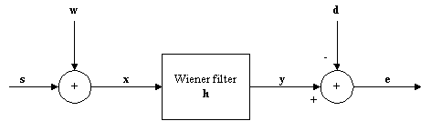
A Wiener filter is a digital filter, which is designed to minimize the mean square difference between the filtered output and some desired signal. It is sometimes called a minimum mean square error (MMSE) filter. This is illustrated in Figure 1, where the difference is the signal e. The original signal is s, the added noise w, and d is the desired signal, which in this application should be equal to s.
In this report I will use matrix-vector notation: Vectors are written in bold and matrices in bold capitals (A). Signals are denoted as vectors (s), samples as scalars with index in the vector (si).

Figure 1: Model for noise reduction problem.
This kind of filter will reduce the noise, as the output y is closer to the evoked potential than the original recording, x.
3.1 Constructing a Wiener filter
Applying the filter h to x can be expressed as a matrix multiplication:
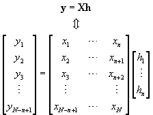 (1)
(1)
Where N is the number of samples in x and n is the number of filter coefficients. We want to find h so that y » d. Using the 2-norm as a measure of difference, that is minimizing the mean square error (MSE), ||e|| equal to the difference
||y – d|| = ||Xh – d||. (2)
From general optimization theory we have
that the solution to the problem ![]() , where X have the same number of rows as d and
the same number of columns as the length of h, can be found by the
normal equation[1]:
, where X have the same number of rows as d and
the same number of columns as the length of h, can be found by the
normal equation[1]:
(XTX)-1XT is called the pseudoinverse of X, as this is equal to solving an overdetermined system. X is very easy to construct and require no computations, just moving some elements around. The desired signal, d, which should be the evoked potential, is of course not known – if it was known we did not need the filter at all. Therefore some approximation to d is needed. This will be discussed later.
XTX is actually an estimate for the autocorrelation matrix of x and XTd the crosscorrelation between x and d (see Appendix 1 for definitions). In some applications it might be easier to estimate the correlations than the actual signals. With the auto- and crosscorrelation matrices R and P, respectively, (3) can be expressed as
h = R-1 P . (4)
3.1.1 Example
The following is a simple example of how X, h and d look for n = 3 and a sequence of five desired output values:
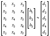 (5)
(5)
The sequence of input values is longer than the output sequence. Often this is achieved by zero-padding when applying a FIR filter to some data sequence.
3.1.2 Filter delay
An ordinary linear phase FIR filter introduces a delay equal to half the filter order because the coefficients are symmetric, and the output sample corresponds in time to the input sample multiplied by the middle filter coefficient. For a Wiener filter, the delay introduced is decided by the time shift between d and x when computing P. If the delay is chosen negative, meaning that the output sample is later in time than the last input sample, it can actually also be used for linear prediction.
In my implementation of this method, x and d have the same length but no zero-padding is performed. Instead some elements in d are simply not used in constructing the filter. Which elements are not used is decided by the specified filter delay. For a filter of length 3 introducing no delay, the first two elements in d are unused.
3.1.3 Effective computation
Finding h by directly calculating the expression in (3) involves several matrix multiplications and a matrix inversion. This takes time and introduces rounding errors in numerical computations. A better way of solving the normal equation is by QR factorization[2].
QR factorization of a matrix X
produces an upper triangular matrix R of the same dimension as X
and a unitary matrix Q so that X = Q·R. In an
“economy size” QR factorization, which is used here, only the first n
columns of Q (denoted ![]() ) are computed meaning that
) are computed meaning that ![]() and X have the
same dimensions. h can now be found by solving the simpler system
and X have the
same dimensions. h can now be found by solving the simpler system
![]() (6)
(6)
This is actually what happens in Matlab when solving an overdetermined system by writing
h = X\d
as done in my implementation.
Note that if the number of filter coefficients is set too high, the rank of the matrix system may be insufficient. This only happens if it is possible to construct a “perfect” filter where the MSE is zero. In that case the number of filter coefficients should be set equal to the rank of X.
A Matlab implementation, which returns h for given x and d, is included in Appendix 2. When using the function, n and the delay should be specified as arguments. It does not, however, support negative delay, as it is not needed in this application, but it would be simple to implement.
3.1.4 Example
A simple test of the method is shown in Figure 2. Here, the source signal s is a high frequency sine wave and the added noise a low frequency sine wave. When s is known we can set d = s to get the optimal filter.
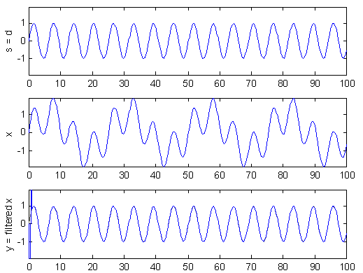
Figure 2: Example use of Wiener filter to remove low frequency noise. The filter output in the bottom plot is almost a perfect reconstruction of the source.
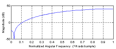
In this example a good results is achieved with only four filter coefficients, i.e. n = 4. The delay is set to zero, which means that the first three samples of filter output are incorrect because x is zero-padded when the filter is applied. As expected for this kind of problem, the filter produced is actually a high pass filter (see Figure 3).
Excluding the first and last few samples, MSE was computed to 2.3523·10-26. Generally, more filter coefficients reduce the MSE but increase the computation time. In this simple example the MSE cannot get any smaller because the system of equations is singular for larger n. It means that the filter is “perfect” for the data and the MSE is only an effect of rounding errors.
|
|
Figure 3: Amplitude response of optimal filter. |
3.2 Epoch optimization by Wiener filtering
As mentioned, some approximation to the true evoked potential is needed to construct a Wiener filter for the EEG epochs. Cichocki et al. (2001) compute a new filter for each epoch setting x to the epoch and d to the average of all the other epochs. The epoch itself is excluded from the average to make the noise in x and d uncorrelated, as the filter will not remove noise that is also present in the approximation, d.
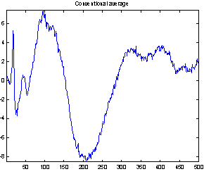
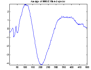
Figure 4 demonstrates the effect of the filtering. It shows both the conventional average and the average of the filtered epochs from a Wiener filter with 50 coefficients. It is not possible to compare the two averages with the true evoked potential to see which is best, as the true response is not available. But the conventional average contains much more high frequency noise, and EEG usually does not have that much high frequency contents, so it seems reasonable to assume that the average of the filtered epochs is the best.
|
|
|


Figure 4: Comparing conventional average and average of MMSE filtered epochs. The example is the evoked response to stimulus 1, Cz electrode on subject 102. 118 epochs were used.
Epoch averaging presupposes that the evoked potentials in all epochs have the same latency. In this kind of experiments small variations can occur, and different approaches for correcting latency jitter exists. MMSE optimized filters should be able to compensate for time differences in an interval corresponding to the filter length, because a filter introducing the necessary delay will result in lower MSE when comparing the filter output to the average d. Hence the Wiener filtering both improve the signal-to-noise ratio and compensate for latency jitter, thereby providing a better basis for the subsequent averaging.
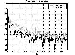
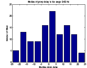
As the noise changes, the filters constructed for each epoch are quite different. The amplitude response of some of the filters used for the demonstration above is shown in Figure 5. They are obviously not just common band pass or band stop filters. Still the filters primarily remove frequency contents greater than 15 Hz, which is visible in the power specters in Figure 6. The histogram in Figure 7 indicates the filters ability to compensate for latency jitter: The median of the filter group delay computed in the frequency interval 0-50 Hz varies around zero.
|
|
|
|
|
|
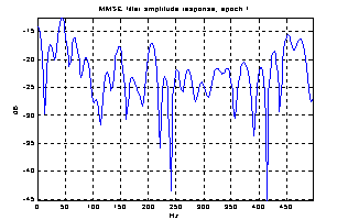

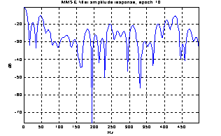

Figure 5: Amplitude response of Wiener filters for four different epochs.
|
Figure 6: Power specters of the two averages. |
Figure 7: Histogram of filter group delay. |
A better way of evaluating the method is to make two estimations of the evoked potential from smaller subsets of the epochs and compare these. In Figure 8 the conventional average and the average of MMSE filtered epochs is shown for two 20-epoch subsets from the 118 epochs used above. The EP might change a little over time, and to compensate for that I excluded the first 20 epochs and selected two sets of every second epoch starting from number 21 and number 22. This way any slow change in the responses over time will not influence the comparison of the subsets, nor will the subjects getting used to the sound in the first few minutes.
The two conventional averages shown to the left are quite different, especially the peaks near sample 25 and sample 400. There are also differences in the filtered averages, but they are less obvious, and these two computed from only 20 epochs seems to be almost as good as the conventional average of all 118 epochs.
|
|
|
|
|
|
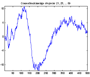

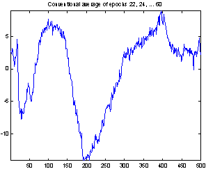
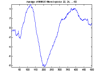
Figure 8: Comparing conventional average and average of MMSE filtered epochs. The example is the evoked response to stimulus 1, Cz electrode on subject 102. 20 epochs were used.
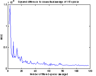
Now,
to get an idea of how many epochs are necessary to achieve results comparable
to those obtained from conventional averaging of 118 epochs, I produced some
plots like the one in Figure
9. Here, the mean value of the squared difference
between normalized versions of the conventional average ![]() and the average of i
Wiener filtered epochs
and the average of i
Wiener filtered epochs ![]() , are plotted for i going from 2 to 118 epochs. The
difference is calculated as:
, are plotted for i going from 2 to 118 epochs. The
difference is calculated as:
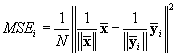 (7)
(7)
The
epochs used for computing ![]() are chosen at random
from the full set of epochs. MSEi is expected to decrease as
the number of epochs increases, until the two ways of extracting the evoked
potential give equally good results. For large i,
are chosen at random
from the full set of epochs. MSEi is expected to decrease as
the number of epochs increases, until the two ways of extracting the evoked
potential give equally good results. For large i, ![]() should be a better estimate than
should be a better estimate than ![]() , and MSEi is almost constant.
, and MSEi is almost constant.
This happens at about i = 20, which like the plots in Figure 8 indicate that with this method only 20 epochs are needed to extract the evoked potential. That is a considerable reduction of the number used for conventional averaging.
|
|
Figure 9: Mean square difference between conventional average and the average of a number of Wiener filtered epochs. |
4 Subspace methods
In my first study of evoked potentials[3], spatial PCA was used to reduce the number of channels to analyze. A similar technique with the purpose of reducing noise in the epochs will be examined here and combined with Wiener filtering.
4.1 Temporal PCA
In data/channel reduction, further analysis is performed of some of the principal components instead of the recording. In this application, the data is reconstructed from a subset of the components. The signals obtained from the electrodes are treated independently, and instead of separation in space the different time epochs are used as input components for the PCA. It means that for 100 obtained epochs, the covariance matrix is 100 x 100 and the output is 100 components.
If an eigenvalue in the analysis is large, many input components have contributed to the corresponding principal component. For 100 components, all principal components with a power contribution of less than 1% to the total power (eigenvalue less than 1 for normalized covariance matrix) can be considered as noise if the same signal is known to exists in all input components. The evoked potential should be present in all epochs, so actually there is only one source in a signal obtained from an electrode and only one principal component should be preserved.
The Matlab function pcareduce in Appendix 3 can discard a number of principal components and then reconstruct the epochs. The principal component fj is discarded simply by setting the samples to zero, fj = 0, before reconstructing by multiplying the components with the inverse transformation matrix. Modifying the inverse transformation matrix instead could save some computations, but this simple approach is sufficiently fast here.
4.2 Alternative approach: SVD
The same kind of noise reduction can be achieved using singular value decomposition. This method is denoted the subspace method, because it divides the data into signal and noise subspaces. The epochs should be arranged as columns in a matrix Y. SVD of Y produce three matrices so that
S has nonnegative diagonal elements in decreasing order; U and V are unitary matrices.
The columns of U are orthogonal, thus subsets of the columns span subspaces of the space spanned by U. As a result, the matrix U can be split into two parts: U = [Us Un], where the columns in Us are associated with the signal and the columns in Un are associated noise part of the epochs. The number of columns in Un is the number of principal components that should be removed in the PCA method, and making Us contain only the first column of U correspond to only using the principal component with the largest eigenvalue.
The signal part is extracted by computing the projection of the observed signals Y onto the signal subspace:
where the columns in Z are the “cleaned” epochs. These are equal to the epochs reconstructed from the reduced set of principal components if the epochs in Y have zero mean. Hence the PCA and the SVD methods can give the same results.
Again, for evoked potentials, Us should be chosen as only the first column of U because there is only one source. When Us is a single column, all the columns in Z are just Us scaled with different constants, because
![]() (10)
(10)
and UsT y is a scalar. The scale is the length of the projection of y onto Us.
4.3 Subspace method and Wiener filtering combined
Cichocki et al. (2001) propose combining the subspace method with Wiener filtering. The subspace method performs best for relative high SNR because this gives better separation between the signal and noise spaces, but EEG recordings typically have low SNR. As mentioned, a Wiener filter cannot remove noise in the frequency bands where desired signal is. But it can increase the SNR, and thus give a better starting point to compute the subspaces.
The proposed method is to do singular value decomposition of the filtered epochs – that is constructing Y and U for (8) from the filter output. The raw signal is then projected onto the signal subspace. With the raw epochs as columns in X, this is:
![]() (11)
(11)
I did some tests with this method similar to the test described for the Wiener filter in section 3.2, and they showed very little difference from just averaging the filter output as in Figure 8. The output was not exactly the same, but I was not able to find any improvement. The only thing the subspace method does when Us is a single column as in this application, is to produce a weighed average of the filtered data instead of a conventional average, and this has no significant effect.
5 Conclusion
Wiener filters both reduce background noise thereby improving the signal-to-noise ratio and compensate for latency jitter in the epochs. It was demonstrated that applying Wiener filters to the recordings can considerably improve the extracted evoked potentials, and in that way reduce the number of epochs required. In my tests the results achieved with only 20 epochs seemed as good as the results from conventional averaging of more than 100 unfiltered epochs.
The subspace methods had little effect on the noise; both used alone and applied after Wiener filtering. An explanation could be that the noise was almost equally powerful in all epochs, which would mean that the weighting of the epochs was almost equal. In that case it is close to a conventional average.
Another way of evaluating the methods might be to use artificial data simulating brain evoked potentials with background noise, where the SNR is known. That could give a quantitative estimate of the improvement in SNR from both the Wiener filtering and the subspace methods.
6 Literature
Aunon, Jorge I., McGillem, Clare D. and Childers, Donald G.
Signal processing in evoked
potential research: Averaging and Modeling
CRC Critical Reviews in Bioengineering
July, 1981
Cichocki, Gharieb and Hoya
Efficient extraction of evoked
potentials by combination of Wiener filtering and subspace methods
Lab. for advanced Brain Signal Processing
Brain Science Institute, RIKEN, 2001
Madsen, Kaj and Nielsen, Hans Bruun
Supplementary Notes for 02611
Optimization and Data Fitting
IMM, DTU, 2002-8-13
http://www.imm.dtu.dk/courses/02611/
Proakis, John G. and Manolakis, Dimitris G.
Digital Signal Processing
Third edition
Prentice Hall 1996
Vinther, Michael
AEP analysis in EEG from
schizophrenic patients using PCA
Ørsted, DTU, 2002-6-7
http://logicnet.dk/reports/
Widrow, Bernard and Stearns D. Samuel
Adaptive Signal Processing
Prentice Hall 1985
Appendix 1 Correlation estimates
The autocorrelation matrix is[4]
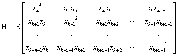 (12)
(12)
and the crosscorrelation is
![]() , (13)
, (13)
where n is the number of filter coefficients wanted. E denotes expected value over any time index, k. The expected value of P can be computed by simple averaging.
R can be computed in several ways. One was described in section 3.1, another is the modified covariance method (a.k.a. forward-backward method). This estimate can be computed by the Matlab function corrmtx. For a length N real-valued signal vector x, it is the matrix product
 . (14)
X is here a 2(N-n+1) by n matrix.
Appendix 2 Wiener filter generator function
%h=mmsefilter(x,d,n,a)
% x Recorded signal
% d Desired signal
% n Number of filter coefficients
% a Delay=look-ahead samples, floor((n-1)/2) if not specified
%
%Construct minimum mean square error (MMSE) filter.
%
% 2002-10-04 | Michael Vinther | s973971@student.dtu.dk
function h=mmsefilter(x,d,n,a)
if nargin<4
a = floor((n-1)/2);end x = x(:)';d = d(:);if size(x,2)~=size(d,1)
error('x and d must have same length');end r = size(d,1)-n+1;if r<n
error('Too few known samples for specified filter order.');end X = zeros(r,n);for i=1:r
X(i,:) = x(i:i+n-1);end h = X\d(n-a:n-a-1+r);
Simple function to apply a FIR filter to a data sequence. The output vector is of same length as the input, and the filter is not mirrored, as it is when conv is used for filtering.
%x=filter1(s,h,a)
% s Data sequance
% h Filter
% a Filter delay=look-ahead samples, floor((n-1)/2) if not specified
%
%1D digital filter. h is not mirrored as with conv,
%and length(x) = length(s).
%
% 2002-9-29 | Michael Vinther | s973971@student.dtu.dk
function x=filter1(s,h,a)
if nargin<3
a = floor((length(h)-1)/2);endx = conv(s,flipud(h(:)));x = x(1+a:a+length(s)); % CropAppendix 3 Functions for noise reduction by PCA
%Noise reduction by discarding principal components
% [F,D,T,n] = pcareduce(S,n)
%
%Input parameters
% S : Matrix with original components in the columns.
% n : Number of principal components to preserve or, if n<1, take
% enough components to get a
fraction n of the total power.
%
%Output parameters
% F : Matrix with new components in the columns.
% D : Vector with component power.
% T : Transformation matrix.
% n : Number of principal components preserved.
%
% 2002-10-05 | Michael Vinther | s973971@student.dtu.dk
function [F,D,T,n] = pcareduce(S,n)
[F,D,T] = pca(S);
if n<1
if n<=0
error('n must be greater than
0')
end
P = D./sum(D)
pn = n;
n = 1;
p = P(1);
while p<pn
n = n+1;
p = p+P(n);
end
end
F(:,n+1:end) = zeros(size(F(:,n+1:end)));
F = (T\F')';
%Principal component analysis
% [F,D,T] = pca(S)
%
%Input parameters
% S : Matrix with original components in the columns.
%
%Output parameters
% F : Matrix with principal components in the columns. The first
column
% contain the component with
the greatest power.
% D : Vector with component power. Each element in D corresponds to a
% column in F.
% T : Transformation matrix so that F = (T*S')'
%
% 2002-10-05 | Michael Vinther | s973971@student.dtu.dk
function [F,D,T] = pca(S)
R = cov(S);
[U,D,V] = svd(R); % SVD returns sorted result with largest eigenvalue
first
D = diag(D)';
T = diag(sqrt(1./D))*V';
F = (T*S')';