1 EEG.. 1

1.1 Oscillation frequencies. 1

1.2 Types of activity.. 2

1.3 Gating.. 3

2 Principal component analysis, PCA.. 5

2.1 Introduction to PCA.. 5

2.2 The eigenvalue problem... 5

2.3 Computation of principal components. 9

2.4 Properties of PCA.. 9

2.5 Implementation.. 10

3 Literature.. 11

Appendix 1     Jacobi implementation.. 13

1 EEG

The usual way of examining a “black-box” system where the parts cannot be separated and examined one by one is to apply some input signal and then analyze the output. One such system is the human brain, where inputs can be applied through our senses: Visual, auditory (hearing), somatosensory (feeling), olfactory (smelling) or gustatory (tasting). In this study output will be the electroencephalogram, EEG.

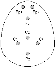
     An EEG is recorded from a number of electrodes placed on the scalp (see Figure 1) and typically the ears are used as ground. At each electrode a superposition of the large number of brain cell (neuron) potentials is obtained. The results are weighed sums, where the weights depend on the signal path from the neurons to the electrodes. Because the same potential is recorded from more than one electrode, the signals from the electrodes are highly correlated. The potentials at the electrodes are in the mV range and therefore very sensitive to noise, so a special designed amplifier/sampler has to be used.

1.1 Oscillation frequencies

The first EEG recorded was alpha rhythms with frequencies about 10 Hz. This was done by Berger (1929), who also found and named beta activity. Beta is today used to describe the frequency range from about 12 Hz to 30 Hz. Experiments show that the amount of alpha activity varies when eyes are closed and opened, see Figure 2. Gamma frequency oscillations (30-80 Hz), which were found by Adrian (1942), are today believed to correlate with binding and attention[1]. Binding is the process of combining sensory input to form the perception of one or more objects.

     In addition to alpha, beta and gamma, the ranges 0.25-4 Hz and 4-7 Hz are respectively named delta and theta. The frequency ranges are not strictly defined, and different papers use slightly different frequency intervals.

Figure 2: Ten seconds of EEG. The subject’s eyes were closed during the first two seconds. The opening of the eyes first result in suppressed alpha activity, and then speeded alpha when the eyes are again closed after eight seconds[2].

1.2 Types of activity

1.2.1 Spontaneous

When recording the response to some stimuli, e.g. a sound, the EEG will always contain some activity that is uncorrelated with the stimuli. This is seen both during and in between stimulations, and is called spontaneous activity. It is caused by processes, which may be unrelated to the experiment being performed.

1.2.2 Evoked

Evoked potentials (EP) are phase-locked to the onset of stimuli meaning that every time the stimulus is applied, they appear at the same latency. Most kinds of sensory stimulation cause evoked potentials. The recordings, which will be analyzed in this report, contain auditory evoked potentials (AEP). These are found within the first 500 ms after stimuli.

     The amplitude of evoked potentials is usually smaller than that of the spontaneous activity, and they are rarely visible in a single recording (see Figure 3). By averaging a number of recordings with the same stimulus, the other activities will cancel out and only evoked potentials remains because they are phase-locked (see Figure 4). In general the signal to noise ratio is improved with the square root of the number of epochs averaged, and with AEPs preferable more than 100 epochs should be used.

1.2.3 Induced

Like evoked potentials, induced potentials are directly caused by the experimental stimuli. But they appear with varying latency or phase, and hence they will be removed by averaging so other methods have to be applied to extract them.

Figure 3: Four EEG channels sampled at 1 kHz. The EOG channel is used to exclude epochs with eye movement. The 50 ms pulses in the event channel signals the onset of a click with duration 1.6 ms  (subject 114).

Figure 4: Average of 117 stimulus pair epoch s. Here, the evoked potentials clearly stand out.

1.3 Gating

Our brain receives a large number of inputs from our senses all the time, and one of its primary tasks is to sort out what is important and what is not. One way of doing that is to focus only on changes. Figure 4 shows the evoked potentials resulting from two click sounds with an interval of ½ second. The response to the second click has much less amplitude than the first response because of this effect, which in this paradigm is called gating.

     The ability to pay attention to the significant is very important to us, and it is an ability that is weakened with schizophrenic patients. Therefore the gating effect should be less visible with schizophrenic patients i.e. the amplitude difference should be smaller[3]. Of specific interest is the early response in the 50 ms latency range, as this is considered preattentive. As such the abnormality in the gating of the early responses could form the basis of the disturbance in attention and cognitive function observed in schizophrenic patients. The consistent findings in medicated patients have been reduced gating. However this has only been seen in one study of unmedicated patients.

1.3.1 Comparing evoked responses

To compare the responses, some way of measuring the size has to be established. Traditionally the amplitude of a specific peak in the EEG has been used, see Figure 5. The peaks are named with a “P” or “N” for positive or negative and the approximate latency is ms at which they appear. As the latencies varies from subject to subject, the peak named N100 can be found after both 95 or 105 ms, so the “100” part should not be seen as exact time but just a convenient name.

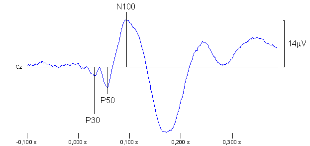
Figure 5: Typical AEP as result of a click at the time 0 s. Note that it is convention to invert the vertical axis when showing EEGs so that peaks with positive voltages point down. Here, 96 epochs from the Cz channel have been averaged to cancel out spontaneous and induced activity (subject 103).

The peaks are very distinct in the example shown here, but in some recordings they can be hard to identify. Often they have to be found by visible inspection, and sometimes they cannot be identified at all. It is very time consuming to do it by hand, but it can be necessary because an automatic peak detection algorithm would make too many errors. Other ways of measuring the size of the responses could be the average power in some time interval or the numerical value of a frequency component in a Fourier transform of the data. The advantage with these approaches is that they can be performed automatically.

     The primary focus in this study has been the preprocessing (averaging, filtering and PCA), and the results presented in the following will be generated by looking at average power.

1.3.2 Frequency bands

Sometimes a band pass filtering can accentuate the response to a stimulus, and often the standard EEG bands (alpha, beta, ...) are used as a starting point for selecting a filter. The evoked potentials shown in Figure 5 have only been high pass filtered with a cutoff frequency of 1 Hz to avoid baseline wander. A band pass filtering preserving e.g. only the gamma band will change the appearance of the potentials considerably, and generally filters with a high lower bound will produce more peaks. Especially when looking at higher frequencies like the gamma band, it becomes more relevant to look at average power instead of comparing peak amplitudes.

2 Principal component analysis, PCA

2.1 Introduction to PCA

PCA is a method to transform a multi-variable data set by a rotation. A rotation is found so that the first axis corresponding to the first component is rotated to the direction where the variance of the data set is greatest. The next component will then be the direction perpendicular to the first with the most variance and so on. Figure 6 show an example with a two-variable data set where the new axes are drawn.

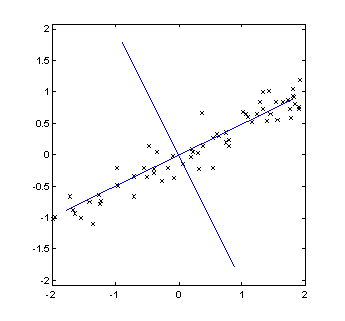
Figure 6, principal components of two-variable data set.

In this application the purpose of PCA is to reduce the number of channels to analyze. In the example it is obvious that most of the variance in the data set is along the first principal component. Assuming that variance equals information contents, one can extract almost all information in the measurement from just one channel.

     The EEG recordings available here have seven channels. Because of the way signals propagate from a source in the brain to the electrodes, large signals will be measured at all electrodes and hence the channels will be highly correlated. The primary interest here is the large signals, as they relative easy can be extracted without too much noise. Therefore PCA is an appropriate tool to reduce the number of channels to analyze. The way it is used here is referred to in the literature as “spatial PCA”.

     The concept of eigenvalues and eigenvectors has to be introduced before describing how to find the transformation, which gives the principal components.

2.2 The eigenvalue problem

l is an eigenvalue of the matrix A_NxN and x the corresponding eigenvector if

                                                                     Ax = xl                                                                     (1)

This can only hold if

                                                                 det|A-lI| = 0                                                                  (2)

Proof of that can be found in any linear algebra book. (2) can be expanded to a N’th-degree polynomial in l, whose roots are the eigenvalues. This means that there is always N eigenvalues, of which some can be equal. For a real, symmetrical matrix the eigenvalues are always real. (1) holds for any multiple of x, but in the following only eigenvectors having length 1 will be considered.

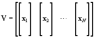
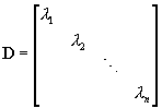
     (1) can be expressed in matrix form with a matrix V whose columns contain the eigenvectors and a diagonal matrix D with the eigenvalues in the diagonal:

                                                                   A V = V D                                                                   (3)

V is orthogonal. This means that all the eigenvectors are perpendicular to each other and hence forms an orthonormal basis. It also means that the transposed of V is equal to it’s inverse:

                                                                     V^T = V^–1                                                                                            (4)

2.2.1 Diagonalization

A matrix A is said to be diagonalizable if a matrix V exists so that

                                                                  D = V^-1 A V                                                                  (5)

is a diagonal matrix. It is obvious that diagonalization is connected to the eigenvalue problem as (3) can be rewritten into (5). If A is already a diagonal matrix, the eigenvalues are simply the values along the diagonal and V is a unit matrix.

     The transformation

                                                                                                                                    (6)

is called a similarity transform. A diagonalization is hence a special case of a similarity transform. It can be shown that a this transform does not change the eigenvalues.

2.2.2 The Jacobi method

The Jacobi method[4] for calculating eigenvalues and -vectors is based on similarity transforms. The transformations are Jacobi rotations of the form

                                                                                    (7)

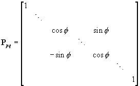
where the diagonal contains ones except for the elements p,p and q,q.  All off-diagonal elements are zero except p,q and q,p. The idea is to do a series of rotations

                                                                                                                                 (8)

which each forces an off-diagonal element p,q in A to zero. It is easily seen thatcan replaceas the inverse rotation of f must be –f and

                                            sin(–f)  = –sin(f) ,       cos(–f)  = cos(f).                                            (9)

Every rotation creates a new zero, but at the same time ruins that created by the previous rotation. The value will, however, be less than the initial value, so by repeated rotations the off-diagonal values will decrease. It can be shown that by repeatedly selecting the numerically largest element and rotating that to, zero one can create a matrix with arbitrarily small values. As the computations in practice are done on a numerical computer with finite precision, the matrix will relatively fast be diagonalized.

     sin(f) and cos(f) can be found by doing the transformation symbolically and setting the expression for  a_pq (element p,q) equal to zero:

                                                                                                                                (10)

                                                                                                                           (11)

                                                                                                                           (12)

                                                                                                                           (13)

where sgn is the sign function: sgn(x) = 1 for x³0 and –1 for x<0.

     The result is a matrix with the eigenvalues in the diagonal. The corresponding eigenvectors are achieved by multiplying all of the transformation matrixes and in that way obtaining the combined transformation:

                                                                                                                              (14)

2.2.3 Example

The eigenvectors and eigenvalues of the following matrix are sought:

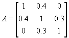                                                                                                                    (15)

The largest off-diagonal element is a₁₂ = 0.4. The rotation, which produces a zero at that position, is found from expressions (10) through (13):

                                                                                                                                (16)

                                                                                                                      (17)

                                                                                                                 (18)

                                                                                                                                 (19)

That gives the rotation matrix

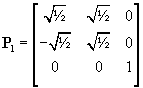                                                         .                                                        (20)

The result of the first similarity transform is then:

                                                                              (21)

Now two elements are numerically equal. One can e.g. continue with a₁₃:

                                                                                                          (22)

                                                                                           (23)

                                                                                                  (24)

                                                                                             (25)

Inserted into (7) this gives the rotation

                                                                                                        (26)

                                                                               (27)

Now after two rotations it is clear that the off-diagonal elements have decreased. After five similar rotations the result is

                                                                                  (28)

If two decimals are sufficient, the matrix is then diagonalized. The eigenvectors can now be found as the combined transformation:

                                                                    (29)

2.2.4 Implementation

The method just described is implemented in the Matlab program in Appendix 1. A practical implementation is usually a little different. The search for the largest value is time consuming. Therefore all the elements are usually just selected systematically one at a time, and when all off-diagonal elements have been the target of the rotation, the selection is restarted. This requires a few more rotations, but these can be done faster. By exploiting that fact that the matrix is always symmetric one can also save a lot of computations[5].

2.3 Computation of principal components

The first component is found as the least mean square error fit to the entire data set. The next component is a least mean square error fit to the residue from the first fit and so on. The transformation matrix that gives this least mean square fit proves to be the matrix, which diagonalizes the covariance matrix of the data (apart from scaling)[6].

     For N channels, the covariance matrix R is an N ´ N symmetrical matrix. The elements are defined as:

                                                                                                    (30)

S is the data set with T samples and  denotes the mean of channel i. If the channel power is normalized, R will contain correlation coefficients and the diagonal will be ones.

     The matrix V, which diagonalizes R can e.g. be found using the Jacobi method described above.

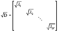
                                                                  D = V^-1 R V                                                                (31)

After the rotation matrix V is found, the principal components, F, can be computed as

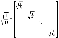
                                                                                                                                 (32)

The factor  is sometimes omitted if scaling of the new components is arbitrary. It is defined as

                                                                                                      (33)

2.4 Properties of PCA

2.4.1 Signal power

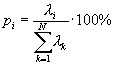
The eigenvalues of R corresponds to the power contribution of the principal components to the data set:

                                                                       l_i = P_i                                                                     (34)

This means that the first principal component is the one corresponding to the largest eigenvalue. For that reason the eigenvalues and eigenvectors are often sorted by power so that l₁ is the first principal component.

     The size of the eigenvalues is an important property when selecting how many channels should be included in the analysis, and how many are to be thrown away. Usually the power contribution from each component in percent is calculated:

                                                                                                                         (35)

One can then include enough channels to preserve e.g. 90% of the total signal power. In the present application, the seven EEG channels can be reduced to two containing about 90% of the original signal power. This is described in detail later.

2.4.2 Noise reduction

In addition to reducing the number of channels, the signal to noise ration can also be improved. As mentioned above, the signal from one powerful source is recorded at all electrodes. The new channels after the PCA transformation/rotation are actually weighed averages of the original channels, and averaging is a well-known method for noise reduction.

     PCA has many applications in digital signal and image processing. One purpose is data reduction or compression as is the case here. Anther is noise removal and reconstruction. The data can be reconstructed from the principal components using the inverse transformation:

                                                                                                                                  (36)

                                                                                                    (37)

If some components with little power are assumed only to contain unwanted noise, they can be removed prior to the reconstruction. In that way the data is restored without the unwanted noise.

2.4.3 Component interpretation

PCA does not necessarily create channels corresponding to the original signal sources when used on a system where signals from different sources are mixed. It just collects as much variance as possible is as few channels as possible. Therefore one cannot expect that the PCA will separate signals from different parts of the brain or that it will separate the EEG from noise coming from sources outside the brain. To achieve such separation independent component analysis, which produces non-orthogonal transformations, could be applied. This is a more complicated method, which will not be described here.

2.5 Implementation

The effect of PCA on a highly correlated data set is demonstrated with the Matlab program in Figure 7 on the next page. The program uses the function JacobiEig shown in Appendix 1 for calculating eigenvalues and –vectors. It demonstrates both the scaled and unscaled rotation using equations (30) through (33). To the right of each program segment of is shown the plot resulting from the code.

     For analyzing the EEG data, an Object Pascal[7] implementation of the algorithm was made. In this implementation the scaled rotation was used, and the Jacobi method was optimized as described in 2.2.4[8].

% Create data with correlated channels

x = (rand(100,1)-0.5)*2.2;

S = [1.6*x x+randn(100,1)*0.25]';

plot(S(1,:),S(2,:),'kx')

% Compute covariance matrix

R = cov(S'); 

% Find eigenvectors and -values

[V,D] = JacobiEig(R); 

% Show new axes         

hold on

A = 2*V';

plot([-A(1,1) A(1,1)],[-A(1,2) A(1,2)])

plot([-A(2,1) A(2,1)],[-A(2,2) A(2,2)])

% Rotate data without scaling

F = V'*S;

figure

plot(F(1,:),F(2,:),'kx')

% Extract diagonal with eigenvalues

d = spdiags(D,0);

% Rotate and scale data

F = diag(sqrt(1./d))*V'*S;

figure

plot(F(1,:),F(2,:),'kx')

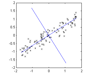
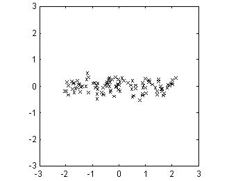
Figure 7: Demonstration of PCA with a highly correlated two-dimensional data set.

3 Literature

Arnfred, Sidse M.; Chen, Andrew C.N.; Eder, Derek N.; Glenthøj, Birthe Y. and Hemmingsen, Ralf P.

A mixed modality paradigm for recording somatosensory and auditory P50 gating

Clementz, Brett A. and Blumenfeld, Laura D.

Multichannel electroencephalographic assessment of auditory evoked response suppression in schizophrenia

Glaser, Edmund M. and Ruchkin, Daniel S.

Principles of Neurobiological Signal Analysis

Hellesen, Bjarne and Larsen, Mogens Oddershede

Matematik for Ingeniører, bind 3

DTU, Institut for Anvendt Kemi

Herrmann, Christoph S.

Gamma activity in the human EEG

Press, William H.; Teukolsky, Saul A.; Flannery, Brian P. and Vetterling, William T.

Numerical Recipes in Pascal: The art of scientific computing

Press, William H. et al.

Numerical Recipes: The art of scientific computing

Proakis, John G. and Manolakis, Dimitris G.

Digital Signal Processing

Third edition

Prentice Hall 1996

Appendix 1      Jacobi implementation

The following program is a simple Matlab implementation of the Jacobi method for finding eigenvalues and eigenvectors. The primary purpose of the program is to demonstrate the method and hence it is not optimized for speed and it is not suited for badly scaled problems.

%[V,D] = JacobiEig(A) returns a diagonal matrix D with eigenvalues and

%a matrix V whose columns are the corresponding eigenvectors so that

%A*V = V*D.

function [V,D] = JacobiEig(A)

Size = size(A,1);

E = eye(Size);

V = E; % Start with unit matrix

for Rotations=[1:Size^2*20] % Limit number of rotations

  % Find maximum off-diagonal element

  Max = 0;

  for r=1:Size-1

    for c=r+1:Size

      if abs(A(r,c))>Max % New Max found

        p = r; q = c;

        Max = abs(A(r,c));

      end

    end

  end

  % Compare Max with working precision

  if Max<eps

    break % A is diagonalized, stop now   

  end

  % Find sin and cos of rotation angle

  theta = (A(q,q)-A(p,p))/(2*A(p,q));

  t = 1/(abs(theta)+sqrt(theta^2+1));

  if theta<0

    t = -t;

  end

  c = 1/sqrt(t^2+1);

  s = t*c;

  % Build rotation matrix

  P = E;

  P(p,p) = c;

  P(q,q) = c;

  P(p,q) = s;

  P(q,p) = -s;

  % Do rotation

  A = P'*A*P;

  V = V*P;

end

D = diag(spdiags(A,0)); % Return diagonal